Artificial Intelligence in Pathology
Article information

Abstract
As in other domains, artificial intelligence is becoming increasingly important in medicine. In particular, deep learning-based pattern recognition methods can advance the field of pathology by incorporating clinical, radiologic, and genomic data to accurately diagnose diseases and predict patient prognoses. In this review, we present an overview of artificial intelligence, the brief history of artificial intelligence in the medical domain, recent advances in artificial intelligence applied to pathology, and future prospects of pathology driven by artificial intelligence.
Artificial intelligence (AI) denotes the intelligence presented by some artificial entities including computers and robots. While AI has only recently received such a large amount of attention, the idea of mechanical thinking can be found in the earliest myths and literature [1]. In the modern era, efforts to model the logical thinking process have continued, and a conceptual machine that is capable of performing arbitrary logical computations was proposed by Turing in 1950 [2]. He believed that the ultimate form of AI would be indistinguishable from humans, and proposed the Turing test as an evaluation method for the intelligence level of machines; this test later faced a number of refutations, including the Chinese room argument in 1980 [3]. In early 2000, Russell and Norvig [4] suggested the concept of an intelligent agent that can automatically plan and perform a series of actions to achieve a goal as a new form of AI, and recently this has been the major focus of AI research.
Several approaches have been taken in the history of AI research [1,4,5]. The first is the human brain simulation approach, in which the human brain is modeled as a network of artificial neurons that receive input signals, process them, and transmit new signals to succeeding neurons. The perceptron is one simple form of such an artificial neural network for recognizing patterns. Symbolic AI is another one that uses symbols and relations to represent human knowledge and uses logical rules to deduce new knowledge to solve intellectual problems. Expert systems are the major product of such an approach, and they have received considerable attention from the industry. Another notable form of artificial neural network is the soft computing approach, including fuzzy logic systems and evolutionary algorithms. This approach has worked well for problems where a sub-optimal, approximate solution is sufficient. The last approach is the statistical learning approach, which relies on statistical data analysis to gather inherent rules that are implicitly represented in raw data. In spite of its lack of explainability, the statistical learning approach is currently the dominant AI research methodology, backed by the success of deep learning.
Deep learning (DL) is a subfield of machine learning (ML) that is based on neural networks comprising several nested layers of neurons. ML, which can be regarded as an alias of statistical learning, is a method of creating a task-specific statistical model from a given dataset. It has been used successfully in several data mining and pattern recognition tasks, including loan default prediction and spam mail filtering [6,7]. Typical ML tasks require domain-specific feature modeling to extract effective information from raw data with the knowledge of domain experts, followed by statistical modeling and learning steps. Linear and logistic regression models, tree-based decision models, and support vector machines (SVM) are famous statistical models that are frequently involved in ML tasks. The major difference between DL and ML is that DL can be done in an end-to-end manner without the feature modeling steps, which tend to be tedious. In DL, appropriate feature models can also be learned from data into the form of convolution filters or multi-dimensional embedding vectors.
The success history of DL begins in the field of visual object recognition. In the ImageNet large-scale visual recognition challenge (ILSVRC) 2012, Krizhevsky et al. [8] demonstrated the excellent performance of their convolutional neural network (CNN), which outperformed the traditional computer vision-based approaches. In 2015, Google DeepMind published a paper about an AI that could learn a human-level control of several Atari 2600 games by trial and error [9], which inspired the AI research community with the idea of deep reinforcement learning. It was somewhat shocking when AlphaGo beat the professional Go player Lee Sedol by 4–1 in 2016 because the game of Go had been regarded as too complex to be well played by the computer for a long time. Moreover, AlphaGo Zero showed that it could beat the AlphaGo 2016 with a > 90% win rate without any prior human knowledge about the game of Go [10]. Speech recognition is another major field of AI research. While several good features and methods had been devised to transform speech signals into text, Baidu Research presented Deep Speech, which showed that an end-to-end DL method could work very well in the speech recognition domain, obtaining a 16.0% word error rate, as compared to an 18.4% error rate for the previous state of the art technology [11]. Automatic translation of text between different languages is one of the most difficult natural language processing tasks, where attention-based recurrent neural network (RNN) models have been successfully applied to get bilingual evaluation understudy (BLEU) scores of 25.9 and 26.3, respectively, in English-to-German translation [12,13]. The more complex task of visual question answering (VisualQA), where textual questions are answered based on a given image or video, has been pursued since its proposal in 2015 [14]. A recent study showed promising results, with accuracy near 62%, as compared to a human’s accuracy of 83% [15].
CNN and RNN are the two most famous DL models for pattern recognition tasks, the former for images and the latter for sequential data like audio and text. Typical CNNs are composed of several convolutional layers followed by a few fully connected layers and a task-specific output layer [16]. High-performance CNN models have more complicated structures that incorporate much more convolutional, pooling, and normalization layers; skip connections and residual connections; branching and merging, etc. An example of modern CNN architecture is shown in Fig. 1. The GoogLeNet is one such model that won the ILSVRC 2014 with a top-5 error rate of 6.67% [17]. RNNs have a special ability to maintain their hidden state in their recurrent layers, which can be regarded as a summary of all their previous input elements. A typical recurrent layer is depicted in Fig. 2, where the input sequence is processed element-wise along with the current hidden state, updating the hidden state and producing the output for the current input element [18]. Long shortterm memory (LSTM) [19] units are a kind of recurrent neuron that has additional learnable gates to prevent itself from losing important information on the input element that was given much earlier; LSTM units are a major component in modern RNN architectures.
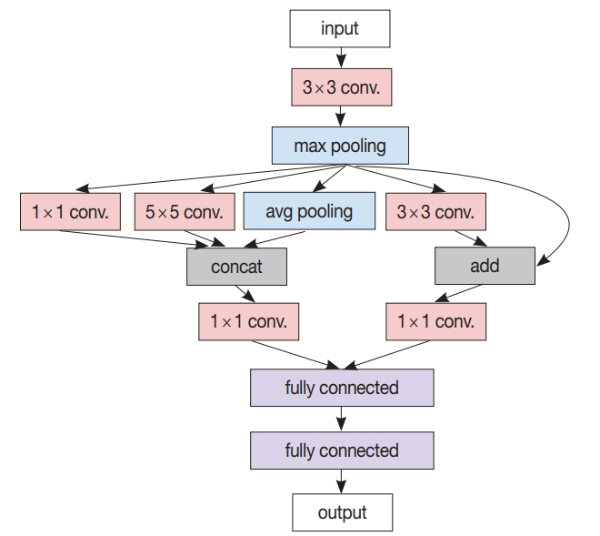
A simplified modern convolutional neural network (CNN) architecture example. In contrast to the classic CNN comprising only a cascade of convolution layers and pooling layers followed by a few fully connected layers, this example has various other concepts like branching from the max pooling layer to several (1×1, 3×3, 5 × 5) convolution layers as well as the average pooling layer, merging by concatenation from two (1×1, 5×5) convolution layers and the average pooling layer, and residual addition of max pooling layer output to the output of its succeeding (3×3) convolution layer.
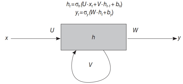
A typical recurrent layer example. In receiving a new input xt at time t, hidden state ht is updated based on xt and the previous state ht-1 first, then output yt is generated based on ht. At training time, parameters like U, V, W, bh, and by are trained to accurately generate yt for every time t.
The list of important terms and abbreviations appearing in this paper is given in Table 1.
List of terms and abbreviations appearing in this paper
HISTORY OF ARTIFICIAL INTELLIGENCE IN MEDICINE
Since the earliest stage of modern AI research, substantial efforts have been made in the medical domain. A script-based chatbot named ELIZA was proposed in 1966 [20]. ELIZA’s most famous script, DOCTOR, could interact with humans as a Rogerian psychotherapist. A biomedical expert system, MYCIN, presented in 1977, could analyze infectious symptoms to derive causal bacteria and drug treatment recommendations [21]. Later, in 1992, the probabilistic reasoning-equipped PATHFINDER expert system was developed for hematopathology diagnosis, to deal with uncertain biomedical knowledge efficiently [22,23].
Before the era of DL, several ML methods have been used widely in the medical domain. Moreover, the invention of digital medical imaging such as digital X-ray imaging, computed tomography and magnetic resonance imaging enabled computerized image analysis, where AI achieved another success in the medical domain. In 1994, Vyborny and Giger [24] reviewed the efforts to use ML algorithms featuring computer vision in several mammography analysis tasks, including microcalcification detection, breast mass detection and differentiation of benign from malignant lesions. They demonstrated the efficacy of computer-aided detection (CAD) by comparing the performance of radiologists with CAD to that of radiologists only. Later, in 2001, Kononenko [25] overviewed the typical ML methods such as decision trees, Bayesian classifiers, neural networks, and k nearest neighbor (k-NN) search, then reviewed their use in medical diagnosis and proposed evaluation criteria including performance, transparency, explainability and data resiliency. In 2003, however, Baker et al. [26] pointed out that the performance of commercial CAD systems was still below the expectation (max case sensitivity 49%) in detecting architectural distortion of breast mammography.
After the success of deep CNN in image classification, a wide range of attempts were made to apply DL to medicine. A notable success was the work of Gulshan et al. [27] in 2016, where retinal fundus images were analyzed by a CNN-based DL model to detect diabetic retinopathy lesions, achieving an area under the receiver operating characteristic curve (AUC) of 0.991, sensitivity of 97.5% and specificity of 93.4% in the high sensitivity setting, measured on the EyePACS-1 data set. In 2017, Litjens et al. [28] reviewed major DL methods suitable for medical image analysis and summarized more than 300 contributions in the neuro, retinal, pulmonary, breast, cardiac, abdominal, and musculoskeletal areas as well as in the digital pathology domain; contributions were well categorized according to their inherent type of image analysis: classification, detection, segmentation, registration, etc. Kohli et al. [29] presented another review on the application of ML to radiology research and practice, where transfer learning and data augmentation were emphasized as a viable solution to datalimited situations. Shaikhina and Khovanova [30] proposed another solution for a similar situation; their proposed solution incorporates multiple runs and the surrogate data test, which exploits statistical tools to guide the trained ML model having better model parameters and not being overfitted to a small training data set.
Genomics and molecular biology have been strongly connected to the medical domain since genome sequencing became real. Next-generation sequencing (NGS) technology allows a whole genome sequence to be translated into text composed of ATCG, so that necessary computational analysis can be done for disease diagnosis and therapeutic decision making. In 2016, Angermueller et al. [31] reviewed DL methods and their application to genomic and biological problems such as molecular trait prediction, mutation effect prediction, and cellular image analysis. They thoroughly reviewed the whole process used to apply DL to their problems, from data acquisition and preparation to overfit avoidance and hyperparameter optimization. Torkamani et al. [32] presented a review of high-definition medicine, which is applied to personalized healthcare by using several kinds of big data, including DNA sequences, physiological and environmental monitoring data, behavioral tracking data and advanced imaging data. Surely, DL techniques can help in analyzing those big data datasets in parallel, to provide exact diagnosis and personalized treatment. Another review was done in 2018 by Wainberg et al. [33] on the use of DL in various biomedical domains, including quantitative structureactivity relationship modeling for drug discovery and identification of pathogenic variants in genome sequences. They re-emphasized the importance of the performance, transparency, model interpretability and explainability of DL methods, in earning the trust of stakeholders gaining adoption. Besides these reviews, there exist two notable contributions for genetic variants. Xiong et al. [34] presented a computational model for gene splicing, which can predict the ratio of transcripts with the central exon spliced in, within the whole set of transcripts spliced from any given sequence containing an exon triplet. Recently an award-winning deep CNN-based variant caller named DeepVariant was announced [35], which is able to call genetic variation in aligned NGS read data by learning on images created upon the read pileups around putative variant sites.
Another type of medical data to be analyzed is electronic health records (EHR). Rajkomar et al. [36] recently published their work building a DL model that predicts multiple medical events, including in-hospital mortality, unplanned readmission, and prolonged length of stay, entirely from raw EHR records based on the Fast Healthcare Interoperability Resources format. Their model could accurately predict mortality events, with an AUC of 0.90 at patients’ admission, and even with an AUC of 0.87 at 24 hours before admission to the hospital. EHR data can be used in the prediction of other types of events, e.g., outcome of a patient biopsy, which could be predicted with AUC 0.69 in the work of Fernandes et al. [37]
Besides the analytical diagnostic tasks, AI has been tried in other areas, for example, an intelligent assistant named Secretary-Mimicking Artificial Intelligence that helps in the execution of a pathology workflow was presented by Ye [38]. Treatment decision is another important factor in patient healthcare, from both prognostic and financial perspectives. Markov decision analysis is an effective tool in such situations, which was used to solve the cardiological decision problem in the work presented by Beck et al. [39] Schaefer et al. [40] reviewed the medical treatment modeling using the Markov decision process, which is a modeling tool that fits well in the optimization of sequential decision making and is strongly related to reinforcement learning [41].
ARTIFICIAL INTELLIGENCE APPLICATION IN PATHOLOGY
Microscopic morphology remains the gold standard in diagnostic pathology, but the main limitation to morphologic diagnosis is diagnostic variability in bearing error among pathologists. The Gleason grading system is one of the most important prognostic factors in prostate cancer. However, significant interobserver variability has been reported when pathologists have used the Gleason grading system [42,43]. In order to get a consistent and possibly more accurate diagnosis, it is natural to introduce algorithmic intelligence in the pathology domain, at least in the morphological analysis of tissues and cells. With the help of digital pathology equipment varying from microscopic cameras to whole slide imaging scanners, morphology-based automated pathologic diagnosis has become a reality. In this review, we focus on morphology-based pathology: diagnosis and prognosis based on the qualitative and quantitative assessment of pathology images. Typical digital image analysis tasks in diagnostic pathology involve segmentation, detection, and classification, as well as quantification and grading [44]. We briefly introduce typical techniques used for AI in digital pathology and a few notable research studies per disease. The list of studies reviewed in this paper is given in Table 2.
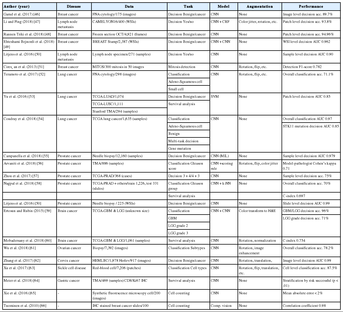
List of research works in applications of artificial intelligence to image analysis based pathology
TYPICAL TECHNIQUES
Digital pathology images used in AI are mostly scanned from H&E stained slides. Pathology specimens undergo multiple processes, including formalin fixation, grossing, paraffin embedding, tissue sectioning, and staining. Each step of the process and the different devices and software used with the digital imaging scanners can affect aspects of the quality of the digital images, such as color, brightness, contrast, and scale. For the best results, it is strongly recommended to alleviate the effect of these variations before using the images in automated analysis work [45]. Normalization is one of the techniques used to reduce such variations. Simple linear range normalization based on the equation [vnew = (vold-a)/fscale + b] is generally used for the pixel values in grayscale images, or for each channel of color images [47,60]. Scale normalization has not been reported in related works, as they all have used a single image acquisition device, e.g., a certain microscopic camera or digital slide scanner. When multiple image acquisition devices are used, scale normalization is of concern, since images acquired from different devices can have different pixel sizes, even at the same magnification level.
Detecting the region-of-interest (ROI) has been done by combining several computer vision operations, such as color space conversion, image blurring, sharpening, edge detection, morphological transformation, pixel value quantization, clustering, and thresholding [67]. Color space conversion is often done before pixel clustering or quantization, to separate chromatic information and intensity information [53]. Another type of color space conversion targets direct separation of color channels for hematoxylin (H), eosin (E) and diaminobenzidine from stained tissue images to effectively obtain nuclei area [57,59,66,68]. Thresholding based on a certain fixed value leads to low-quality results when there are variations in luminance in the input images. Adaptive thresholding methods like hysteresis thresholding and Otsu’s method can generate better thresholding results [47,53,59,69]. Recently, pixel-wise or patch-wise classifiers based on CNN have been used widely in ROI detection [44,49-51,54-56,58,65], where a deep CNN is trained to classify the type of target pixel or patch centered on the larger input image patch in a sliding window manner. Semantic segmentation CNN is another recent trend for this task [65,70,71], which can detect multiple ROIs in a given image without sliding window operation, resulting in much faster speed.
In the development of a CNN-based automated image analysis, data-limited situations are common in the medical domain, because it is very costly and time-consuming to build a large amount of annotated, high-quality data [45]. As previously mentioned, transfer learning and data augmentation should be incorporated to get a better result. In transfer learning, convolutional layer parameters of a CNN, pre-trained with a well-known dataset like ImageNet, are imported into the target CNN as layer initialization, while later layers like fully connected layers or deconvolutional layers are initialized randomly [62,70,71]. Additional training steps can update all of the layer parameters, including the imported ones, or only the parameters of the layers that were randomly initialized. With sufficient data, building a model without transfer learning is reported to give better performance [54].
A common strategy of image data augmentation is, for the given image, applying various transformations that do not alter the essential characteristics; such transformations include rotation (90°, 180°, and 270°), flipping (horizontal/vertical), resizing, random amounts of translation, blurring, sharpening, adding jitters in color and/or luminance, contrasting histogram equalization, etc [47,51,52,56,60-63]. Another type of augmentation relates to the patch generation strategy; applying large medical images directly to the CNN is impractical. From a large pathological image, with a size between 1024 × 1024 (camera) and > 104 × 104 (scanner) pixels, smaller patches with sizes between 32 × 32 and 512 × 512 pixels are retrieved for use in training and inference of CNNs. Instead of using the pre-generated set of image patches through the whole training process, resampling patches during each training epoch can introduce more variance in training data to reduce the chance of overfitting [60].
After the patch-level CNN is trained, another ML model is often developed for the whole image level decision. In this case, a patch-level decision is made for every single patch in the training images to generate heatmap-like output, from which several features are extracted via conventional image analysis methods. Then, collected feature values for the training images are fed into the target image level ML model. An example workflow for developing and using this two-stage pathology AI is depicted in Fig. 3.
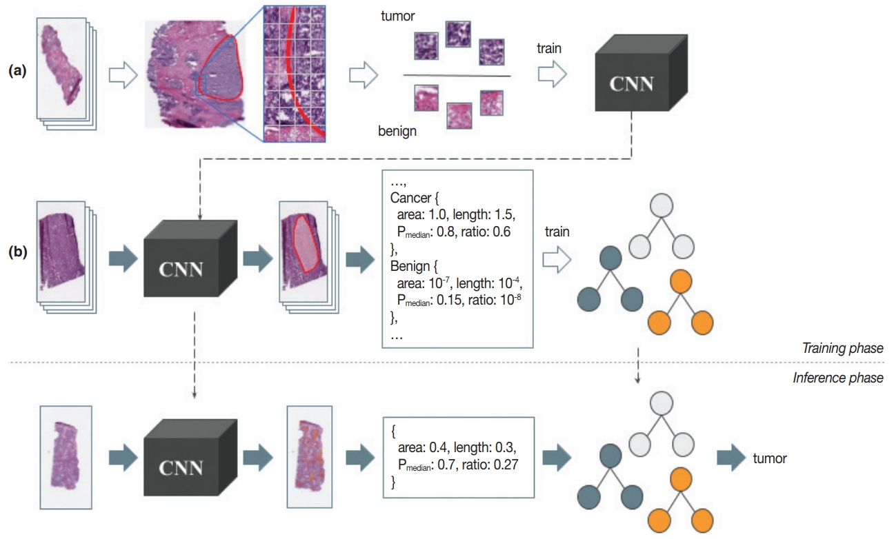
An example workflow for two-stage pathology artificial intelligence. Training phase: from the collected pathology images, a proper amount of annotation data is constructed (a). Image patch sets of balanced size are used in the training of patch-level convolutional neural network (CNN). After the patch-level CNN is trained sufficiently, heatmaps are generated for another set of pathology images using that CNN, from where the features are extracted for the decision forest like image-level machine learning (ML) model training (b). Inference phase: patch-level CNN runs on every single patch in the input pathology to generate a heatmap (first stage). Features are then extracted as in the training phase, and fed into the image-level ML model to determine the image-level result (second stage).
EXAMPLES OF PATHOLOGY ARTIFICIAL INTELLIGENCE
CNN-based breast cancer diagnosis was tried with fine needle aspiration (FNA) cytology images [46], optical coherence tomography (OCT) images [48], and H&E stained tissue images [49], each with varying numbers of data points and model structures. A total of 175 cytology images captured by a microscopic camera at 40 × magnification level were manually split into 918 ROIs, 256 × 256 pixels in size, where each ROI had multiple cells [46]. A CNN was trained to determine the malignancy of a given ROI, and the cytological image was classified as malignant when > 30% of the ROIs in the image were malignant. The reported accuracy was 89.7%, which was far inferior to the 99.4% accuracy of a random forest classifier with 14 hand-crafted features. In order to attempt an automated intraoperative margin assessment, 4,921 frame images from the frozen section OCT were used, from which patches 64 × 64 pixels in size were extracted, resized to 32 × 32 pixels, and used for training and evaluation [48]. Patch-level CNN performance was measured, giving an accuracy of 95.0% and AUC of 0.984 in the best setting. In another study, 2,387 H&E stained breast biopsies were scanned at a magnification of 20 × [49]. Multiple CNNs were used in this study: the first CNN classified each image pixel as fat, stroma, or epithelium; the second CNN predicted whether each stromal pixel was associated with a cancer; and the third CNN determined the whole-slide-level malignancy. The reported slide level AUC was 0.962. A notable result is that, while the CNNs were trained with stromal tissues in benign slides and invasive cancer slides only, the predicted cancer association probability of the stroma near the ductal carcinoma in situ (DCIS) lesion properly related to the severity of DCIS. CNN-based lymph node metastasis detection was also tried with a different model and dataset [47,50]. Conditional random field was adopted on top of convolutional layers in order to regulate the metastasis prediction [47]. From the whole slide images (WSIs) in the CAMELYON16 dataset [72], benign and tumor image patches 768 × 768 pixels in size were sampled to train and validate the model, giving patch-level accuracy of 93.8% after incorporating data augmentation methods. In another study, 271 WSIs scanned at a magnification of 20 × were used in developing a CNN-based model for detecting micro- or macro-metastasis-free slides [50]. Region-level annotations on training images were utilized. Slide-level metastasis detection was performed after metastasis probability map generation by patch-level CNN, incorporating probability thresholding (> 0.3) and connected component analysis to remove small lesions (< 0.02 mm diameter), resulting in a detection AUC of 0.90. Mitosis detection was tried with a CNN that decides whether the center of the given image is mitotic or not [51], trained and evaluated with 50 images from five biopsy slides containing about 300 mitoses total, adopting data augmentation techniques including patch rotation and flipping. In the evaluation, a mitosis probability map was created for the given image, and pixels with locally maximal probabilities were considered as mitotic, resulting in detection F1-score 0.782.
Automatic lung cancer subtype determination was tried with FNA cytology images and H&E stained WSIs [52,54]. A total of 298 images from 76 cases acquired using a microscopic camera at 40 × magnification level were utilized in developing a CNN receiving 256 × 256 pixel images as input; the dataset comprised 82 adenocarcinomas, 125 squamous cell carcinomas, and 91 small cell carcinomas [52]. Data augmentation techniques like rotation, flipping, and Gaussian filtering were adopted to enhance the classification accuracy from 62.1% to 71.1%. A total of 1,635 WSIs from the The Cancer Genome Atlas (TCGA) [73] dataset were used in detection of lung cancer type with CNN [54]. Each input patch (512 × 512 pixels) was classified as adenocarcinoma, squamous cell carcinoma or benign, and then the averaged probability of non-benign patches was used in the slide-level decision, resulting in slide level classification AUC of 0.97, which is much superior to the previous SVM-based approach [53]. Moreover, by using the multi-task transfer learning approach, mutations of six genes including KRAS, EGFR, and STK11 were independently able to be determined on the input WSI of lung adenocarcinoma patches. The mutation detection had an AUC of 0.86 for STK11 and an AUC of 0.83 for EGFR.
Prostate cancer diagnosis has been one of the most active fields in adopting DL because of its large dependence on tissue morphology. Prostatic tissues from various sources have been used in malignancy and severity decisions [50,55-58]. In one study, 225 prostate needle biopsy slides were scanned at 40 × magnification, and malignant regions were annotated in developing a cancer detector [50]. A CNN-based patch-level cancer detection was performed for every overlapping patch in a slide to generate a probability map, and a cumulative probability histogram was created and analyzed in slide-level malignancy determination (AUC 0.99). In another study, 12,160 needle biopsy images were utilized in developing a CNN-based slide-level malignancy detector [55]. To train a patch-classifying CNN with no patch/regionlevel manual annotation, multiple instance learning was used; with a large number of WSIs (> 8,000), the result was useful (AUC 0.98). A total of 886 tissue microarray (TMA) samples were used in a trial of automated Gleason scoring [56], where 508 TMA images for training were manually segmented into combinations of benign, Gleason pattern 3, 4, and 5; 133 TMA images were used for tuning and 245 images were used for validation. The TMA level score was determined by the two most dominant patterns measured from the per-pattern probability maps generated by a trained patch-level CNN classifier. In grading the validation set, Cohen’s kappa between two pathologists was 0.71, while those between the model and each of the two pathologists were 0.75 and 0.71. 342 cases from TCGA, teaching hospital and medical lab were utilized in training automated Gleason scoring system [58], where CNN and k-NN classifier were ensembled. A total of 912 slide images were annotated with the region level to be used in training CNN to generate a pattern map for a given slide image; 1,159 slides were used to train the k-NN classifier that determines the Gleason group for the given pattern map statistics. The reported grading accuracy measured on 331 slides was 0.70, while the average accuracy of 29 general pathologists was 0.61, which is superior to the previous TCGA-based result that showed 75% accuracy in discriminating Gleason score 3 + 4 and 4 + 3 [57].
An automated determination of brain cancer severity was tried with TCGA brain cancer data [59]. A cascade of CNNs was used: an initial CNN trained with 22 WSIs for discriminating between glioblastoma (GBM) and low-grade glioma (LGG), and a secondary CNN trained with an additional 22 WSIs for discriminating between LGG grades 2 and 3. Each H&E-stained RGB color image was transformed into an H-stained channel and an E-stained channel, and only the H-stained channel was used for further analysis. The first CNN showed GBM/LGG discrimination accuracy of 96%, but the LGG grade discrimination was not so successful (71%). Survival analysis using CNN was also tried [60]. Again, 1,061 WSIs from TCGA dataset were used. For each training epoch, 256 × 256 pixel patches were sampled from manually identified, 1,024 × 1,024 pixel ROIs. At diagnosis, ROI-wise risk was determined as the median risk of nine patches sampled from the ROI, and the sample-level risk was determined as the second highest risk among ROI risks. The measured c-index of this kind of survival analysis was 0.75, which was elevated to 0.80 by modifying the CNN to receive the mutation information at its fully connected layer.
Ovarian cancer subtype classification based on CNN was tried [61]. 7,392 images were generated by splitting and cropping the original images acquired by the microscopic camera at 40 × magnification level. Rotation and image quality enhancement were used in the data augmentation phase, which enhanced the classification accuracy from 72.8% to 78.2%. Cervical cancer diagnosis on cytological images was also tried [62]. Without cell-wise segmentation, nuclei-centered cell patches were sampled from the original cytology image, followed by augmentation operations like rotation and translation. Convolutional layer parameters that were trained by using ImageNet data were transferred to actual CNN. Herlev and HEMLBC datasets were used in evaluation, giving 98.3% and 98.6% accuracy, respectively, in five-fold cross-validation. Red blood cell (RBC) classification is crucial in sickle cell disease diagnosis. A CNN-based automatic RBC classification was tried [63], where 7,206 cell patches were generated from 434 microscopic images and used for training and testing of the classifier. Rotation and flipping were used to augment training data. Five-fold cross-validation showed an average accuracy of 89.3% in five-class coarse classification, and 87.5% in eight-class refined classification. A total of 469 TMA cores from the gastric cancer patients were used in a CNN-based survival analysis [64]. CD8 and Ki67 immunostained images were acquired and fed into separate patch-wise risk-predicting CNNs for each stain. From the differential analysis between the low-risk group and the high-risk group, it was claimed that the density of CD8 cells was largely related to the risk level.
FUTURE PROSPECTS
We have provided an overview of various medical applications of AI technology, especially in pathology. It is encouraging that the accuracy of automated morphological analyses has improved due to DL technology. The pathologic field in AI is expanding to disease severity assessment and prognosis prediction. Although most AI research in pathology is still focused on cancer detection and the grading of tumors, pathological diagnosis is not simply a morphological diagnosis, but is a complex process of evaluation and judgment of various types of clinical data that deal with various organs and diseases. A large amount of data, including genetic data, clinical data, and digital images, is needed to develop AI that covers the range of clinical situations. There are a number of public medical databases, including TCGA, and a number of studies have been done based on those databases. They provide a good starting point in researching and developing a medical AI, but it requires much more high-quality data; e.g., detailed annotations on a large number of pathology images, created and validated by several experienced pathologists, are necessary to develop a pathology-image-analyzing AI that is comparable to human pathologists.
There are difficulties in constructing such high-quality data in reality, largely due to the protection of privacy, proprietary techniques, and the lack of funding and pathologists to participate in the annotation process. To overcome this data insufficiency, as we have mentioned earlier, several techniques have been introduced, such as transfer learning and data augmentation. Still, these techniques are sub-optimal; transfer learning cannot guarantee the optimal convolutional filters specific for the task, and data augmentation cannot deal with the unseen data and patterns. The ultimate solution is to construct a large amount of thoroughly labeled and annotated medical data, through the cooperation of multiple hospitals and medical laboratories. To accelerate the construction of such a dataset, efficient tools for labeling and annotating are required, which can be assisted by another type of AI [45].
Eventually, there will be a medical AI of the prognostic prediction model, combining clinical data, genetic data, and morphology. Also, a new grading system applicable to several tumors can be created by an AI model that has learned from the patient’s prognosis combined with a number of variables including morphology, treatment modality, and tumor markers, etc. This will also help to overcome the poor reproducibility and the variety of current grading and staging results among pathologists, leading to much better clinical outcomes for patients.
Notes
Conflicts of Interest
The authors declare that they have no potential conflicts of interest.
Acknowledgements
This study was approved by the Institutional Review Board of The Catholic University of Korea Seoul St. Mary’s Hospital with a waiver of informed consent (KC18SNDI0512).